Nearest Neighbor
|
|
Number, Spatial distribution |
Nearest Neighbor investigates the 3D spatial arrangement of objects such as cells within thick sections of a region of interest. |
|
|
|
Thick |
||
|
|
Any |
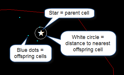
Stereo Investigator records the (X,Y,Z) coordinates of "parent cells" and of neighboring "offspring cells." From this coordinate data, Stereo Investigator calculates the nearest neighbor distance for each parent cell and the nearest neighbor distributions for the region of interest.
The Nearest Neighbor analysis is performed within the context of a systematic random sampling of the tissue; this means that a counting frame size and XY grid spacing between counting frames must be defined for each specimen.
Once the Nearest Neighbor probe is started,Stereo Investigator drives the stage to each counting frame location and displays a standard counting frame.
- Within each counting frame, each parent cell is marked.
- A scan is performed through the entire Z-depth of the counting frame and each cell close to a parent cell is marked as an offspring cell.
- Stereo Investigator calculates the shortest distance to determine the closest offspring cell for each parent cell.
- An Optical Fractionator analysis is automatically performed on the parent cell population to generate an estimated total number of the parent cell population for the region of interest to be included with the Nearest Neighbor results.
See Optical Fractionator prerequisites.
Place a representative slide under the microscope, navigate to the region of interest using a low magnification lens, place a reference point.
The magnification should be high enough to clearly distinguish individual cells, but low enough to display each cell’s nearest neighbor in the same field of view.
![]() Displaying the nearest neighbor be in the same field of view is not a requirement, but it will save significant time in the survey.
Displaying the nearest neighbor be in the same field of view is not a requirement, but it will save significant time in the survey.
Click Probes>Define Counting Frame and set the size and location of the counting frame.
- Select a low magnification lens and draw a closed contour around the region of interest.
- Use Probes>Preview SRS Layout. Stereo Investigator displays an aerial view of the contour with a grid of counting frames overlaying it.
If the total number of counting frames is too large, use larger values for the X and Y SURS Grid Size.
- If there are not enough counting frames, use smaller values.
- Click anywhere in the tracing window to dismiss the aerial preview display of the SRS layout.
- Switch to a high power lens suitable for counting cells (the one used to define the counting frame size); remember to select this lens from the list on the Stereo Investigator toolbar.
- Select a marker for counting parent cells.
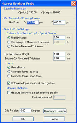
- Click Probes>Nearest Neighbor. The Nearest Neighbor Probe dialog box opens
 with the values determined during the Preview SRS Layout operation entered. Make any changes if needed.
 - Enter the guard zone height under Distance From Section Top to Optical Disector field.
(Guard Zone height * 2) + Optical Disector Height <= minimum Mounted Thickness.
- If you have very uneven tissue thickness within each section, check Measure section thickness at each selected grid site.
- Stereo Investigator will prompt you to identify the top and bottom of the section at each scan site. Thickness is recorded and used to report Number Weighted Section Thickness results which take into account the varying thickness in calculating your final estimated total.
- Click OK in the Nearest Neighbor Probe dialog box. Stereo Investigator randomly selects the starting point of the scan and moves the stage to the first counting frame (a random starting point is necessary to insure unbiased sampling).
- Stereo Investigator displays the Focus Top of Section dialog box. Identify the top then click OK.
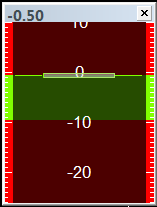
- If you selected Measure section thickness at each selected grid site, the Focus Bottom of Section dialog box opens. Identify the bottom then click OK. Stereo Investigator automatically moves the stage to the top of the counting frame. If the focus position meter is enabled, you will see the Z-axis extent of the counting frame in green
 . When the cursor is above or below the counting frame height, the cursor is shown as an objective lens with a slash through it to indicate that cells should not be counted outside of the counting frame height.
- If you selected Measure section thickness at each selected grid site, the Focus Bottom of Section dialog box opens. Identify the bottom then click OK. Stereo Investigator automatically moves the stage to the top of the counting frame. If the focus position meter is enabled, you will see the Z-axis extent of the counting frame in green
- Mark the first parent cell within the 3D counting frame. The counting frame is no longer visible.
- Focus through the full depth of the tissue and mark all offspring cells that are in proximity to the selected parent cell. Stereo Investigator uses a default marker for the offspring cells.
- As each offspring cell is clicked, Stereo Investigator draws a white circle around the parent cell with a radius of the distance to the nearest offspring cell
 .
.
 If a new offspring cell is further away from the parent cell than a previously marked offspring cell, the radius of the circle does not change.
The radius of the circle changes as you focus up and down because it represents a sphere around the parent cell.
The offspring cells do not need to be located within the counting frame, which is why the counting frame is not displayed. - As each offspring cell is clicked, Stereo Investigator draws a white circle around the parent cell with a radius of the distance to the nearest offspring cell
- Once all offspring cells in proximity to the parent cell have been marked, right-click and select Next Parent Cell. The counting frame is displayed again, and another parent cell can be marked.
- All cells that are located within the 3D counting frame must be defined as parent cells.
- If two parent cells are offspring cells of one another, the circle drawn around the second parent cell is automatically drawn with a radius of the distance to the first parent cell.
- Once all parent cells have been defined and their offspring cells marked, the analysis is complete for that counting frame. Press F2 to go to the Next Scan Site.
- Repeat steps 7 through 11 until you have examined all of the counting frames distributed across the region of interest for this section.
- Verify that the number of cells counted is close to, or somewhat larger than, the target number of cells (for a single section).
To see the number of markers counted:
- Select Probes>Display Probe Run List, highlight the most recent Nearest Neighbor run and click the View Results button.
OR
- From the Markers toolbar, right-click and select Show Marker Summary.
- Return to a low magnification lens and move the stage so that a new section is visible.
- Define a new section in the Serial Section Manager. Stereo Investigator enters the values from the first section are used for section thickness, Z-depth and section name but you may edit them if necessary.
- Trace a contour around the region of interest in the new section.
- Switch to a high power lens for counting, and click Probes>Nearest Neighbor. Stereo Investigator displays the Nearest Neighbor dialog box with the values used in the first section.
![]() Do not change these values for a new section in the same specimen.
Do not change these values for a new section in the same specimen.
- Click OK to begin counting. The stage is moved to the location of the first counting frame.
- Continue as above for the remaining sections of this specimen.
![]() The counting parameters can vary across specimens, but they must remain the same for every section in a given specimen in order to extract valid CE data.
The counting parameters can vary across specimens, but they must remain the same for every section in a given specimen in order to extract valid CE data.
- Select Probes>Display Probe Run List.
- Click the View Results button; Stereo Investigatordisplays the Sampling Results in the right pane of the dialog box.
- Click a Marker name on the left for marker counts and estimates of total number.
Typically each marker is used to represent one cell type. If an optical fractionator is being used to count multiple types of cells, a different marker type should be used to identify each cell type.
Displays the file name associated with this data set if the data has been saved to or read from a file.
Displays the data and time when the probe was completed.
Displays the name of the contour type that defines the region of interest over which the probe was implemented.
If a composite of several runs is being examined, Stereo Investigator displays the contour name used for the first run.
Number of sampling sites visited on all selected sections.
Area of the contour bounding the regions of interest or sum of areas (for composite of multiple optical fractionator runs).
Stereo Investigator calculates this area from the geometry of the bounding contour(s). This area can be compared to the area determined using the Cavalieri Probe.
Area of a single counting frame.
Thickness of the counting frames along the Z-axis.
Volume of a single counting frame.
X-axis width of each counting frame (in microns).
Y-axis height of each counting frame (in microns).
Represents the distance between counting frames (sampling sites) along the X-axis.
Represents the distance between counting frames (sampling sites) along the Y-axis.
Area of the region that is associated with each sampling step.
Value used for section thickness across all sections that were sampled.
Should be the minimum actual section thickness as measured by Stereo Investigator.
Number weighted mean of all sections measured by focusing at the top and bottom of the section.
This value should be relatively close to the Section Thickness.
- Click Number Weighted Details for details.
Estimated population count determined by the selected series of optical fractionator runs.
Estimated population count determined by the selected series of optical fractionator runs, using for the section thickness value the number weighted section thickness.
Actual number of markers of this type counted during the optical fractionator survey.
These markers also represent the cells designated as parent cells during the Nearest Neighbor survey.
Raw data of the number of counts for each counting frame visited in each of the runs of the optical fractionator.
Raw data of the nearest neighbor distance for each designated parent cell. The X,Y,Z distance from each parent cell to all designated offspring cells is calculated, and the shortest of these distances reported for each cell.
CRF (cumulative relative frequency) is created from the raw data for the nearest neighbor distances (nnd). For each nnd on the X-axis, the graph shows a Y-value that indicates the probability that any particle would be that distance or less from another particle.
Example CRF Graph and Explanation 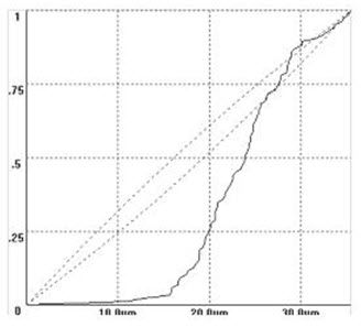
In this example of a CRF graph, the nearest neighbor distances are given on the x-axis. For this discussion, ignore the area delineated by the dotted lines. If you look at a given nnd, you can tell the probability that any particle would be that distance, or less (since it’s a cumulative frequency graph), from another particle. You can use the CRF graph to interpret the 3D arrangement of your particles. For instance, in this graph, there is a scarcity of short distances that indicates a relatively dispersed situation. If we compared this data set to another group of cells that were more clustered, the CRF would rise more rapidly because there are many short distances.
For examples with comparisons of CRF graphs of nnds, see Fig. 2 in Altered Spatial Arrangements (Schmitz et al.) or Fig. 4 in Spatial distribution and density... (Segal et al.). Apply caution when comparing CRF graphs that come from systems with different number of cells and/or different densities.
Shows the probability that a cell anywhere in the tissue will be located within a given distance of another cell (i.e., will have a particular nearest neighbor distance).
The maximum distance shows a probability of 1, since all cells will be within that distance or less of their nearest neighbor.
Diggle (1983). Statistical analysis of spatial point patterns. London, Academic Press.
Schmitz C, G. N., Hof PR, Boehringer R, Glaser J, Korr H. (2002). Altered spatial arrangement of layer V pyramidal cells in the mouse brain following prenatal low-dose X-irradiation. A stereological study using a novel three-dimensional analysis method to estimate the nearest neighbor distance distributions of cells in thick sections." Cereb Cortex 12(9): 954-960.
Segal D, S. C., Hof PR. (2008). Spatial distribution and density of oligodendrocytes in the cingulum bundle are unaltered in schizophrenia. Acta Neuropathol 117(4): 385-394.
Stereo Investigator 11 | MBF Bioscience Support Center | Downloads