Cavalieri Estimator Probe
|
|
Volume |
Use for a quick and efficient estimation of the area and/or volume of a region of interest. Stereo Investigator overlays a regular grid of points on the slide/image; you mark the points in the grid that lie over the region of interest. Volume of a structure = Total number of points marked * Distance between points in XY * Distance between points in Z |
|
|
|
Preferential sections |
The Cavalieri Estimator is a grid of dimensionless points randomly placed on the region of interest to be estimated. With a grid, the intersections of each of the grid lines are related to the areas formed by the grid.
By associating one area with a point (more accurately, a dimensionless point) located at each intersection, the entire area of the grid is represented.
Each point represents a given area. Because it is not possible to draw a dimensionless point, we represent this concept as a cross or plus sign, where a unique feature of the cross (such as the lower left quadrant of the cross) is used to consistently mark the points which overlay the region of interest 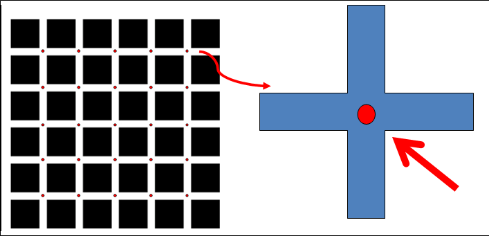 .
.
You need to determine an appropriate distance between the points of the point grid that will be overlaid on the region of interest.
The grid spacing determines the number of markers placed.
- Smaller grid spacing results in a more precise estimate, but requires placing more markers.
- Larger grid spacing saves time, but may result in reduced precision.
It is up to you to find the right balance between precision and efficiency. The more points you have, the more decisions you have to make.
![]() Based on theoretical and practical experienceHoward and Reed, Unbiased Stereology, First Edition, p. 41, we know that you can obtain a volume estimate with a 10-15% coefficient of error from 10-15 evenly spaced systematic random sections through the region of interest, and a grid spacing that results in ~200 marker points in total (not per section).
Based on theoretical and practical experienceHoward and Reed, Unbiased Stereology, First Edition, p. 41, we know that you can obtain a volume estimate with a 10-15% coefficient of error from 10-15 evenly spaced systematic random sections through the region of interest, and a grid spacing that results in ~200 marker points in total (not per section).
For volume estimation, you also need to know either the thickness of the sections to be sampled, or the thickness interval between the sections to be sampled.
- Place a reference point.
- Select the lens that matches the objective from the drop-down menu in the toolbar.
- Use Tools>Serial Section Manager to define sections.
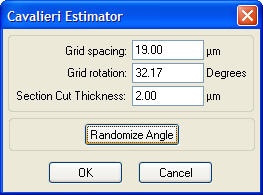
- Click Probes>Cavalieri Estimator; the Cavalieri Estimator dialog box appears
 .
.- Section Cut Thickness: Defined in the Serial Section Manager.
- Grid spacing: Enter a value.
- Click OK; Stereo Investigator displays a grid of points (represented by cross-hairs by default) over the tissue.
- To change the shape and color of the grid points, use the Options>Stereology Preferences>Colors And Tick Marks tab.
- Click a marker type in the toolbar to select it.
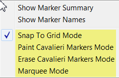
- Snap To Grid is the default marking mode. To select another marking mode, place the cursor over the tracing window and right-click
 (see Cavalieri Estimator - Marking Modes)
 - Mark all the points that overlay the area of interest on the section.
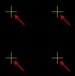
- Use the same unique point for each grid point when determining whether the grid point is over the area of interest.
- Use different markers for different sub-regions.
 If the grid point is represented by a cross-hair, always approach from the same quadrant.
- Move to the next section.
- Repeat steps 7–9 until all regions on all sections have been evaluated.
- After all of the intersections have been marked, uncheck Probes>Cavalieri Estimator to end the probe run.
- To view the results, use Probes>Display Probe Run List.
|
Snap to Grid Default mode for placing markers |
To mark a point, click in the vicinity of a grid point(+): your marker is placed exactly on the center of the grid point . To place markers in clusters (rather than one at a time), right-click and select Paint Cavalieri Markers Mode or Marquee Mode. |
| Paint Cavalieri Markers Mode |
The cursor looks like this To mark a cluster of grid points, drag the mouse over the area of interest. To adjust the size of the circular cursor, use the "+" and "-" keys of the numerical keypad on your keyboard OR use the mouse wheel. |
| Erase Cavalieri Markers |
|
| Marquee Mode |
To place a cluster of markers within a rectangular area:
To delete a cluster of markers within a rectangular area:
|
| Paint Markers Into Contours |
To fill a contour with markers:
To remove all the markers from a contour, right-click again and select Erase Markers into Contours. The contour must be accurately traced to the boundaries of the region of interest. If not, manually add or remove markers around the edges of the contour. |
| Replace Mode |
To replace a marker type:
|
 .
.You can estimate the area of a 2D structure or the cross-sectional area of a 3D structure.
Both the estimated area of the region of interest and an estimated CE (see Coefficients of Error) for this estimate can be determined from the number of points counted and the known spacing between points.
Volume estimation of regions that are contained in serial sections entails, first of all, the estimation of the volume seen in the individual sections of the serial section sequence.
- An individual section's volume is estimated as the estimated cross-sectional area of the section (as seen at the top or bottom of the section) multiplied by the thickness of the section.
- The estimated volume of the region is the sum of all the individual section volumes.
When the number of sections through the region of interest is large, marking the area of each section becomes a tedious task. The Cavalieri probe facilitates such a task as it is designed to work from a systematic random sample of the sections and will automatically provide information about the area of each section. If the distance between sections is constant, the area estimates of multiple sections can be combined to give an estimate for total volume and a coefficient of error (see ).
![]() Verify that your microtome, cryostat, or other sectioning tool has been properly calibrated prior to sectioning. Typically, you will want to enter the block advance (pre-shrinkage cut thickness) for the section thickness when prompted, not the post-shrinkage mounted section thickness.
Verify that your microtome, cryostat, or other sectioning tool has been properly calibrated prior to sectioning. Typically, you will want to enter the block advance (pre-shrinkage cut thickness) for the section thickness when prompted, not the post-shrinkage mounted section thickness.
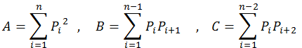
| Area associated with a point |
|
|||||||||||
| Volume associated with a point |

|
|
||||||||||
| Estimated volume |
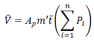
|
|
||||||||||
| Estimated volume corrected for over-projection |
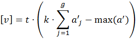
|
|
||||||||||
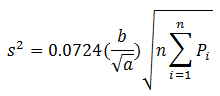
| Variance of systematic random sampling |
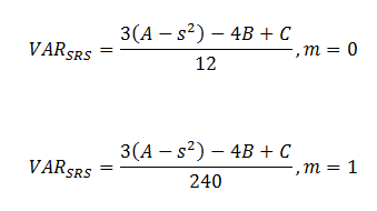
|
|
||||||||||
| Coefficient of Error |
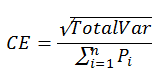
|
|

 where
where  is the shape factor
References
García-Fiñana, M., Cruz-Orive, L.M., Mackay, C.E., Pakkenberg, B., & Roberts, N. (2003). Comparison of MR imaging against physical sectioning to estimate the volume of human cerebral compartments.Neuroimage, 18 (2), 505–516.
Gundersen, H. J. G., Jensen, E.B. (1987). The efficiency of systematic sampling in stereology and its prediction.Journal of Microscopy, 147 (3), 229–263.
Howard, C. V., Reed, M.G. (2005). Unbiased Stereology, Three-Dimensional Measurement in Microscopy (chapter 3). New York: Garland Science/BIOS Scientific Publishers.
The program calculates an estimate of the volume that accounts for the over-projection error during sampling. This estimate is calculated by removing the largest cross-sectional area from the volume estimate calculation.
Over-projection
To explain this concept, let’s start with a simple three-dimensional structure like a sphere.
- To estimate the volume that the sphere occupies in each section, multiply the area of the visible circle in each section by the thickness of the section.
- To estimate the volume of the sphere, add each individual volume together.
With few sections through the sphere, there is an overestimation in the estimated sub-volume (A in the illustration). This is called an over-projection error (represented in blue in the illustration).
As the number of sections through the sphere approaches infinity, the over-projection error decreases (B in the illustration); of course, if you ever managed to get to infinity, the error would be zero. 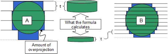
Thus the size of the error depends on the relative ratio of the size of the object and the thickness of the sectioning. It also depends on where the object appears in the section (the error is larger if the object does not extend all the way through the section).
You cannot eliminate the error completely, but in biological experiments, it is often possible to section the tissue thinly enough to get many sections through the area of interest. This is also why it is cumbersome to use the Cavalieri probe on small objects such as cells—it is too laborious to obtain many sections. But note that different methods exist for the estimation of small objects (e.g., Nucleator).
Using systematic random sampling, the error can be reduced even more. If we section the sphere as we did in B above, but only examine every other section (the solid lines in C in the illustration below), the error is smaller than if the section thickness were greater (e.g. A). 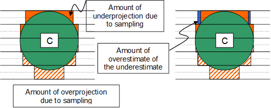 When sampling, the amount of overestimation is balanced by the amount of underestimation. The remaining is known as the “amount of overestimate of the underestimate.”
During sampling, underestimation occurs as the region gets larger as you progress through the sections (solid orange in C above), while as the region decreases in size, overestimation occurs (striped orange in C). The error that remains when you balance the over- and underestimates together is the “overestimate of the underestimate” which is represented by blue in A.
![]() Remember, the amount of over-projection error that may occur in your estimate is due to the variable shape of the region of interest and the number of sections you have through it.
Remember, the amount of over-projection error that may occur in your estimate is due to the variable shape of the region of interest and the number of sections you have through it.
Practically speaking, over-projection error is often considered minimal if you calculate a volume estimate generated from 10-15 evenly spaced systematic random sections through the region of interest.
A more important consideration for the accuracy of the estimation is the definition of boundaries that do not have explicit outlines.
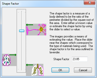
The shape factor is the perimeter of the contour around the area of interest divided by the square root of the area. It is a component of the formula used to calculate the coefficient of error (Coefficients of Error). Stereo Investigator does not calculate a shape factor; instead, it defaults to the value 4.0.
If you determine the shape factor of the areas you are estimating by measuring or estimating the mean area and boundary for your regions, you can modify the shape factor constant used in the CE equation to see the impact on the CE calculation.
![]() Modifying the shape factor does not change the estimated area or volume; it only alters the CE of the estimated area or volume.
Modifying the shape factor does not change the estimated area or volume; it only alters the CE of the estimated area or volume.
Determining a shape factor?
Choose a shape factor on the basis of how the region compares to other shapes:
- Click Move>Where Is to get an aerial view of the region of interest.
- Click Probes>Display Probe Run List.
- Click the View Results button. The Sampling Results dialog box opens.
- Click the Edit Shape Factor button. The Shape Factor dialog box opens
 . After changing the shape factor, the calculations that depend upon it are automatically updated.
OR
Calculate and enter the average shape factor.
- Define the boundary then use the estimate of areas.
- If you have contours traced, you can find the Shape Factor for each contour used in the Contour Measurements window (Contour Measurements).
![]() The Contour Measurements window also contains area information for the contour. Be aware that this information is calculated assuming that the tracing is accurate to the nearest pixel. Use of the Cavalieri method is required to obtain an unbiased estimate.
The Contour Measurements window also contains area information for the contour. Be aware that this information is calculated assuming that the tracing is accurate to the nearest pixel. Use of the Cavalieri method is required to obtain an unbiased estimate.
![]() Consult our Cavalieri Estimator pdf guide.
Consult our Cavalieri Estimator pdf guide.
![]() Watch our webinar Stereological Techniques for Area & Volume Estimation.
Watch our webinar Stereological Techniques for Area & Volume Estimation.
![]() Learn more about a related probe: Area Fraction Fractionator.
Learn more about a related probe: Area Fraction Fractionator.
Stereo Investigator 11 | MBF Bioscience Support Center | Downloads